04-denoise-1d
Basic Introduction to Machine Learning: 04-denoise-1d
Illustrate 1D signal denoising using Julia's Flux library
- Jeff Fessler, University of Michigan
- 2018-10-23 Julia 1.0.1 version
- 2023-01-29 Julia 1.8.5 version
This page was generated from a single Julia file: 04-denoise-1d.jl.
In any such Julia documentation, you can access the source code using the "Edit on GitHub" link in the top right.
The corresponding notebook can be viewed in nbviewer here: 04-denoise-1d.ipynb, and opened in binder here: 04-denoise-1d.ipynb.
Setup
Packages needed here.
using LinearAlgebra: norm, I
using Random: seed!
using Distributions: Normal, randperm
import Flux # Julia package for deep learning
using Flux: Dense, Conv, Chain, SkipConnection, Adam, mse, relu, SamePad
using LaTeXStrings # pretty plot labels
using Plots: plot, plot!, scatter, scatter!, histogram, histogram2d, default, font, gui
using MIRTjim: jim, prompt
using InteractiveUtils: versioninfo

default(markersize=5, markerstrokecolor=:auto, label="")
default(tickfontsize=10, legendfontsize=11)
The following line is helpful when running this file as a script; this way it will prompt user to hit a key after each figure is displayed.
isinteractive() ? jim(:prompt, true) : prompt(:draw);Training data
Generate training and testing data; 1D piece-wise constant signals
Function to generate a random piece-wise constant signal
function makestep(; dim=32, njump=3, valueDist=Normal(0, 1), minsep=2)
    jump_locations = randperm(dim)[1:njump]
    while minimum(diff(jump_locations)) <= minsep
        jump_locations = randperm(dim)[1:njump] # random jump locations
    end
    index = zeros(dim)
    index[jump_locations] .= 1
    index = cumsum(index)
    values = rand(valueDist, njump) # random signal values
    x = zeros(Float32, dim)
    for jj in 1:njump
        x[index .== jj] .= values[jj]
    end
    x[index .== 0] .= values[njump] # periodic end conditions
    x = circshift(x, rand(1:dim, 1)) # random shift - just to be sure
    return x
end
makestep (generic function with 1 method)Training data
seed!(0)
siz = 32

ntrain = 2^11
Xtrain = [makestep(dim=siz) for _ in 1:ntrain] # noiseless data
Xtrain = hcat(Xtrain...) # (siz, ntrain)

ntest = 2^10
Xtest = [makestep(dim=siz) for _ in 1:ntest] # noiseless data
Xtest = hcat(Xtest...) # (siz, ntest)

p0 = plot(Xtrain[:,1:14], label="")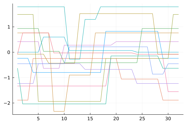
prompt()Data covariance
Kx = Xtrain * Xtrain' / ntrain
p1 = jim(Kx, title="Kx", color=:cividis);
Add noise
σnoise = 0.3
Ytrain = Xtrain + σnoise * randn(Float32, size(Xtrain)) # noisy train data
Ytest = Xtest + σnoise * randn(Float32, size(Xtest)) # noisy test data
Ky = Ytrain * Ytrain' / ntrain;

@show maximum(Kx)
@show maximum(Ky)

p2 = jim(Ky, title="Ky", color=:cividis)
plot(p0, p1, p2, layout=(3,1))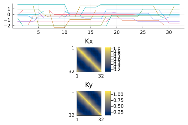
prompt()Wiener filter (MMSE estimator)
# cond(Kx + σnoise*I)
Hw = Kx * inv(Kx + σnoise^2 * I)
jim(Hw; title="Wiener filter", color=:cividis)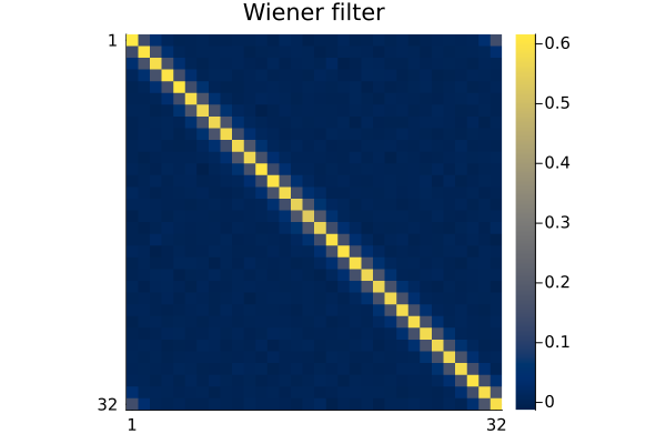
Denoise via Wiener filter (MMSE linear method)
Xw = Hw * Ytest
nrmse = (Xh) -> round(norm(Xh - Xtest) / norm(Xtest) * 100, digits=2)
@show nrmse(Ytest), nrmse(Xw)
colors = [:blue, :red, :magenta, :green]
plot(ylabel="signal value", title="Wiener filtering examples")
for i in 1:4
    plot!(Xw[:,i], color=colors[i])
    plot!(Xtest[:,i], color=colors[i], line=:dash)
    scatter!(Ytest[:,i], color=colors[i], marker=:star)
end
(nrmse(Ytest), nrmse(Xw)) = (30.65, 23.49)prompt()Verify that marginal distribution is Gaussian
histogram(Xtrain[:], label = "Xtrain hist")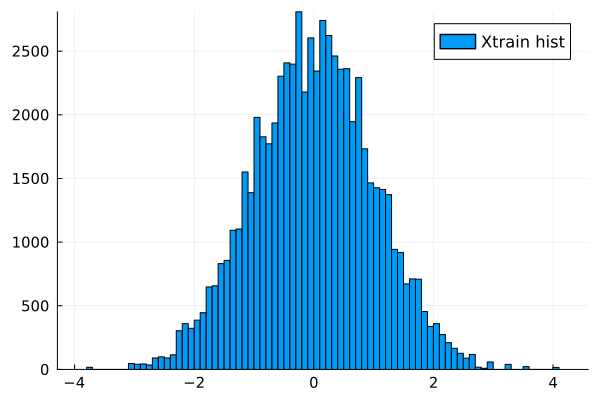
prompt()Simple NN
Examine a "NN" that is a single fully connected affine layer (It should perform same as Wiener filter.)
First try a basic affine NN model
if !@isdefined(state1)
    model1 = Chain(Dense(siz,siz))
    loss3(model, x, y) = mse(model(x), y)

    iters = 2^12
    dataset = Base.Iterators.repeated((Ytrain, Xtrain), iters) # trick X,Y swap for denoising!

    state1 = Flux.setup(Adam(), model1)
    Flux.train!(loss3, model1, dataset, state1)
end;
┌ Warning: Layer with Float32 parameters got Float64 input.
│ The input will be converted, but any earlier layers may be very slow.
│ layer = Dense(32 => 32) # 1_056 parameters
│ summary(x) = "32×2048 Matrix{Float64}"
└ @ Flux ~/.julia/packages/Flux/hrg9M/src/layers/stateless.jl:60Compare training affine NN to wiener filter
H1 = model1(Matrix(I, siz, siz))
jim(H1; title="Learned filter for affine NN", colormap=:cividis)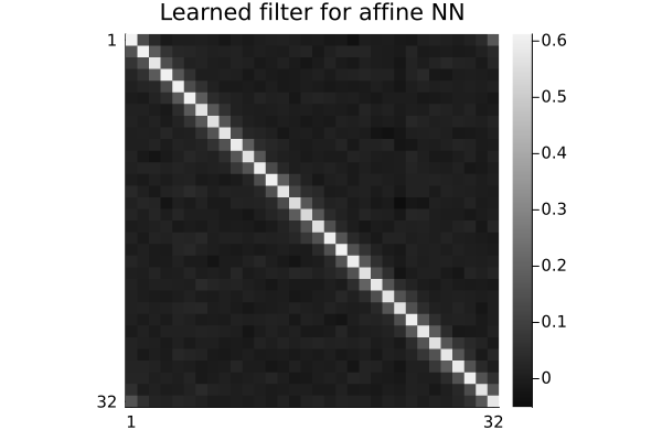
Denoise test Data
X1 = H1 * Ytest
X1nn = model1(Ytest)
@show nrmse(Ytest), nrmse(Xw), nrmse(X1), nrmse(X1nn)
bias = model1(zeros(siz))
@show extrema(bias)
(-0.014208853f0, 0.008303295f0)Examine a single hidden layer NN
Create a basic NN model
if !@isdefined(state2)
    nhidden = 2siz # neurons in hidden layer
    model2 = Chain(Dense(siz, nhidden, relu), Dense(nhidden, siz))

    iters = 2^12
    dataset = Base.Iterators.repeated((Ytrain, Xtrain), iters) # trick X,Y swap for denoising!

    state2 = Flux.setup(Adam(), model2)
    Flux.train!(loss3, model2, dataset, state2)
    X2 = model2(Ytest)
end
tmp = [Ytest, Xw, X1, X1nn, X2]
@show nrmse.(tmp)
5-element Vector{Float64}:
30.65
23.49
25.94
23.66
24.86Examine joint distribution
lag = 1
tmp = circshift(Xtrain, (lag,))
histogram2d(vec(Xtrain), vec(tmp))
plot!(aspect_ratio=1, xlim=[-4,4], ylim=[-4,4])
plot!(xlabel=L"x[n]", ylabel=latexstring("x[n-$lag \\ mod \\ N]"))
plot!(title="Joint histogram of neighbors")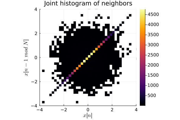
prompt()WIP
Experiments below here - work in progress [https://github.com/FluxML/model-zoo/blob/master/vision/mnist/conv.jl]
if !@isdefined(model3)

    model3 = SkipConnection( # ResNet style: learn residual
        Chain(
            Conv((3,), 1 => 16, relu; pad = SamePad()),
        #  x -> maxpool(x, (2,2)),
            Conv((3,), 16 => 8, relu; pad = SamePad()),
            Conv((1,), 8 => 1, relu),
        #  x -> reshape(x, :, size(x, 4)),
        ),
        +,
    )

    shaper(X) = reshape(X, siz, 1, :) # (siz, channels, batch)
    mymodel3(X) = model3(shaper(X))[:, 1, :]
    @assert size(mymodel3(Xtrain)) == size(Xtrain)

    nouter = 2^2
    ninner = 2^3
    # trick X,Y swap for denoising!
    dataset = Base.Iterators.repeated((shaper(Ytrain), shaper(Xtrain)), ninner)
    for io in 1:nouter
        state3 = Flux.setup(Adam(), model3)
        Flux.train!(loss3, model3, dataset, state3)
        X3train = mymodel3(Ytrain)
        @show io, loss3(model3, shaper(Xtrain), shaper(Ytrain))
        # todo: validation data too
    end
end


X3test = mymodel3(Ytest)
tmp = [Ytest, Xw, X1, X1nn, X2, X3test]
@show nrmse.(tmp) # todo: no improvement!?
6-element Vector{Float64}:
30.65
23.49
25.94
23.66
24.86
27.31Reproducibility
This page was generated with the following version of Julia:
io = IOBuffer(); versioninfo(io); split(String(take!(io)), '\n')12-element Vector{SubString{String}}:
"Julia Version 1.12.6"
"Commit 15346901f00 (2026-04-09 19:20 UTC)"
"Build Info:"
" Official https://julialang.org release"
"Platform Info:"
" OS: Linux (x86_64-linux-gnu)"
" CPU: 4 × AMD EPYC 7763 64-Core Processor"
" WORD_SIZE: 64"
" LLVM: libLLVM-18.1.7 (ORCJIT, znver3)"
" GC: Built with stock GC"
"Threads: 1 default, 1 interactive, 1 GC (on 4 virtual cores)"
""And with the following package versions
import Pkg; Pkg.status()Status `~/work/ismrm_ml2/ismrm_ml2/docs/Project.toml`
[31c24e10] Distributions v0.25.129
[e30172f5] Documenter v1.17.0
[587475ba] Flux v0.16.10
[b964fa9f] LaTeXStrings v1.4.0
[98b081ad] Literate v2.21.0
[170b2178] MIRTjim v0.26.0
[eb30cadb] MLDatasets v0.7.21
[91a5bcdd] Plots v1.41.6
[2913bbd2] StatsBase v0.34.12
[1986cc42] Unitful v1.28.0
[ef84fa70] ismrm_ml2 v0.0.1 `~/work/ismrm_ml2/ismrm_ml2`
[b77e0a4c] InteractiveUtils v1.11.0
[37e2e46d] LinearAlgebra v1.12.0
[9a3f8284] Random v1.11.0This page was generated using Literate.jl.